The impact of macroeconomic variables on asset pricing. An analysis using the APT framework.

This post is quite a bit longer and more technical than my usual blog entries—it's actually my MSc thesis. I'm sharing it for all the macroeconomics enthusiasts out there (like myself), as well as for students who may find it useful. If you choose to cite my work (which would be an honour), please don’t forget to include proper references. I’ve also included a full list of the sources I used at the end of the paper. 🙂

Abstract

This study explores the relationship between macroeconomic variables and stock market returns, analysing monthly data spanning from January 2000 to January 2020. The selected macroeconomic indicators include the consumer price index (as a proxy for inflation), the index of industrial production (as a measure of economic activity), and 10-Year Treasury Bill Rates (as a representation of interest rates). Employing the ordinary least squares (OLS) estimation model, the research aims to uncover the underlying connections between these variables and asset pricing. Empirical findings unveil compelling insights into the interactions between these economic indicators and stock market performance. Notably, a significant positive correlation surfaces between the consumer price index and stock market returns, implying that higher inflation rates correspond with increased stock market returns. Conversely, a weak negative relationship emerges between industrial production and interest rates, suggesting their limited influence on stock returns. These findings hold crucial implications for stakeholders such as corporate managers, investors, and policymakers.

Key words: Stock market returns, inflation, interest rates, industrial production, US.

Acknowledgements

I would like to express my sincere gratitude to my supervisor Konstantinos Tolikas for his insightful mentorship throughout the course of my project.

I am deeply thankful to my parents Artela and Murat, whose endless love, encouragement, and sacrifices have been the foundation of my journey and achievements.

Chapter 1 – Introduction

In today's globalised and interconnected financial systems, understanding the determinants of asset pricing has become a crucial area of research. The relationship between macroeconomic factors and asset prices has long been a subject of great interest for economists, investors, and policymakers alike. Recognising this relationship and its implications for investment decision making is vital for both individual investors seeking to optimise their portfolios and financial institutions aiming to manage risk effectively.

The Arbitrage Pricing Theory (APT) stands as a robust framework employed to explore asset prices and their intricate interactions with a range of macroeconomic factors. Unlike the Capital Asset Pricing Model (CAPM), which focuses primarily on market risk and adopts a one-dimensional approach, the APT takes a comprehensive stance. This comprehensive approach entails considering a multitude of influential factors that influence asset returns, encompassing macroeconomic variables like interest rates, inflation rates, exchange rates, GDP growth, and other pivotal indicators. By adopting the APT framework, this study endeavours to shed light on the complex web of relationships that shape asset prices, thereby contributing to a more holistic understanding of the dynamics driving the asset pricing landscape in the United States.

The central focus of this dissertation revolves around the following research question: How do macroeconomic variables influence asset pricing within the APT framework? This inquiry aims to uncover the complex relationship between macroeconomics and asset valuation, providing insights into the underlying mechanisms that drive the pricing of financial instruments. By examining this relationship, this study’s objective is to expand the existing literature in the field of finance and offer valuable insights that can inform investment strategies, risk management techniques, and policy decisions. In the realm of financial markets, the intricate relationship between macroeconomic variables and asset pricing stands as a pivotal determinant of investment decisions and market dynamics. The United States, as a global financial hub, offers a compelling backdrop to explore this nexus. Over the years, the interplay between various macroeconomic indicators—ranging from inflation rates and interest rates to industrial production—has held a profound influence on the pricing of diverse assets. This study delves into this intricate interrelationship, seeking to unveil the underlying patterns and causal connections that govern how these variables impact the pricing of assets in the U.S. financial landscape. By delving into this vital link, the research aims to provide not only a deeper understanding of the dynamics driving asset prices but also insights that can guide investment strategies and policy formulation in an increasingly complex and interconnected economic environment.

To comprehensively address this research question, the methodology employed involves conducting an empirical analysis that incorporates historical data and statistical modelling techniques such as OLS and unit root testing. The

examination of the past performance of various asset classes in relation to macroeconomic factors aims to identify patterns and determine the extent to which these factors influence asset prices. This investigation requires gathering pertinent data on macroeconomic indicators, namely, inflation, interest rates and economic activity and asset returns from reliable sources such as FRED, constructing econometric models, and conducting statistical tests to validate the hypotheses. Moreover, this study will contribute to the growing body of literature that explores the applicability and effectiveness of the APT framework across different market conditions. While the APT has gained popularity as an alternative to the CAPM, it is crucial to assess its validity and robustness in diverse economic environments. By doing so, we aim to provide practitioners and researchers with a nuanced understanding of the APT's efficacy and limitations, thereby enhancing the tools available for asset pricing and risk management.

In conclusion, the primary objective of this dissertation is to investigate the impact of macroeconomic factors on asset pricing within the APT framework. Through this exploration, this study aims to unveil valuable insights into the interplay between macroeconomics and financial markets. Ultimately, the findings of this study possess the potential to guide investment decisions, shape risk management strategies, and contribute to the broader understanding of asset pricing dynamics in an ever-evolving global economy.

Research Question:

How do macroeconomic variables influence asset pricing in the United States?

Research Objectives:

1. Toexaminetherelationshipbetweenmacroeconomicvariables(suchas interest rates, inflation rates, and industrial production) and stock market returns in the US.

2. Toassesstheimplicationsofthefindingsforinvestmentdecision-making and risk management in the US financial markets.

Chapter 2 – Literature Review

2.1 Theoretical foundations 2.1.1 Asset Pricing Theory

The theory of asset pricing aims to provide explanations and establish pricing mechanisms for financial assets in an uncertain environment. This theory posits that asset prices are not solely driven by market sentiment but are inherently intertwined with a spectrum of risk factors. Among these risk factors, macroeconomic variables play a significant role, exerting their influence through elements such as interest rates, inflation rates, exchange rates, and broader economic indicators. This intricate interplay between asset prices and macroeconomics has prompted the development of various financial models aimed at dissecting these relationships. These models are designed to unravel the intricate web of connections between macroeconomic variables and asset prices, thereby contributing to a more profound comprehension of the intricate interactions shaping the landscape of asset pricing. Through the lens of these models, researchers and practitioners gain a broader insight into how changes in macroeconomic conditions reverberate across asset classes, ultimately informing investment strategies and risk management practices in an ever-evolving financial landscape.

2.1.2 The Capital Asset Pricing Model (CAPM) – An introduction

The foundation of modern asset pricing theory lies in the Capital Asset Pricing Model (CAPM), an influential framework introduced by Sharpe (1964), Lintner (1965), and Mossin (1966). This model serves as a cornerstone in establishing a systematic link between the inherent risk associated with an asset and the potential return it offers. It seeks to quantitatively define the intricate relationship between these fundamental elements. The model's formulation is expressed in a linear equation as follow;

𝑹𝒕 = 𝜶 + 𝜷𝑿𝒕 + 𝜺𝒕 (2.1)

In this equation 𝑅𝑡 represents the return of the asset under consideration, 𝑋𝑡 represents the return derived from an underlying portfolio of assets, reflecting the broader market performance. The component 𝜀𝑡 represents the asset-specific return whereas the Beta (𝛽), represents the index of undiversifiable risk, often referred to as market risk or systematic risk.

The primary objective of utilising CAPM is to decompose a portfolio’s risk into systematic and specific risk. Specific, or diversifiable risk is the type of risk that is unique to an individual asset, and it is not correlated with general market

movements (Ouma and Muriu, 2014). These risks are typically related to internal factors of a specific entity, such as company specific events or developments. For instance, factors like the introduction of a new product, staff performance or customer service relationships can impact the specific risk of an investment. However, the specific risk can be mitigated through diversification, where investors spread their investment across various assets to reduce the impact of individual asset risks (Smart et al. 2017).

On the other hand, systematic risk, is inherent in the overall market and cannot be avoided, therefore all assets have an equal systematic risk and are equally affected by general market movements which are generally caused by broader macroeconomic forces such as economic growth, interest rates, inflation etc., that play pivotal roles in driving systematic risk. For instance, during periods of economic growth the market sentiment tends to be positive, leading to increased investment and consequently higher asset prices. Conversely, increased inflation or interest rates can lead to lower investor confidence, resulting in market downturns and falling asset prices. In CAPM, the beta coefficient is used as a measure to quantify the change of an asset’s return in response to a change in the market return (Aljandali and Tatahi, 2018). Although CAPM has been widely used to understand the relationship between risk and return and the implications of risk on asset pricing, this model does not fully address the complexities of the impact of macroeconomic variables on asset pricing. Its limitation lies in its narrow focus on systematic risk alone. It does not explicitly incorporate the influence of specific macroeconomic variables, such as economic growth, interest rates, inflation, or other fundamental economic indicators that can significantly impact asset pricing. In order to gain a more comprehensive understanding of how macroeconomic variables affect asset pricing, a more advanced, multi-factor model, namely the Arbitrage Pricing Theory (APT) was introduced by Ross in 1976.

2.1.3 Arbitrage Pricing Theory (APT)

The Arbitrage Pricing Theory is an augmentation of CAPM, which was developed to address some of its limitations and provide a more flexible and comprehensive framework for asset pricing. APT is based on a multi-factor linear model which accounts for various measures of systematic risk. An APT model takes the following form:

𝑹𝒕 =𝜶+𝜷𝟏𝑿𝟏𝒕 +𝜷𝟐𝑿𝟐𝒕 +⋯+𝜷𝒏𝑿𝒏 +𝜺𝒕 (2.2)

Equation 2.2 is an extension of equation 2.1, whereby the X’s represents a number of risk factors common to a class of assets and the betas represent the sensitivity of the asset’s return to each factor. This model investigates whether the risk linked to a specific macroeconomic variable is accurately represented in the anticipated market returns.

According to (Chen, Roll, & Ross, 1986), economic variables play a significant role in influencing stock market returns, primarily through their impact on discount rates, a firm’s ability to generate cash, and future dividend payments.

These economic forces can have a systematic effect on the stock market as a whole and not only on the individual stocks. The APT suggests that only a small number of systematic factors significantly influence asset returns over the long run. This means that a few important macroeconomic variables, rather than a multitude of specific factors, drive the general patterns in stock market returns.

(Jecheche, 2006) argues that APT as a multi-factor model allows assets to have multiple measures of systematic risk, capturing their sensitivities to various pervasive factors. In the absence of specific risk, assets move simultaneously and are therefore just leveraged "copies" of one another. This makes it relatively straightforward to assess and predict their returns using APT. However, when assets have specific risk, which is the type of risk that is unique to an individual asset, forming portfolios that combine different assets can help to diversify the specific risk of each asset and therefore reducing its impact on the overall portfolio’s risk. Yet, achieving full diversification of residual risk, which is the risk that cannot be diversified away, is challenging. It requires including an infinite number of securities in the portfolio, which is practically impossible. Therefore, the author concludes that in this case, the APT pricing restrictions only hold approximately.

Chen et al (1986) conducted one of the earliest studies using observed factors and they argue that at the most basic level, the prices of assets, such as stocks, are determined by fundamental valuation models. Specifically, the price of a stock is influenced by the correctly discounted expected future dividends it is expected to generate. Based on this fundamental valuation framework, the authors suggest that when considering risk factors in APT, it is essential to include any systematic influences that impact future dividends. These systematic influences could involve various economic and financial forces that affect the firm's future profitability and performance. Furthermore, the authors point out that the choice of factors should also take into account how traders and investors form expectations and how they discount future cash flows. By accounting for these systematic influences and the way investors respond to economic information, macroeconomic variables become part of the risk factors in the equity market. This implies that changes in macroeconomic variables can have significant effects on stock returns, and these effects can be captured and quantified through appropriate risk factors within the APT framework.

2.2 Empirical Literature

Naik (2013) conducted a study to examine the influence of macroeconomic factors on stock market behaviour using data from India. The analysis utilised monthly data spanning from April 1994 to April 2011, encompassing five key macroeconomic variables: industrial production index, inflation, money supply, short-term interest rate, and exchange rates. To explore the long-run equilibrium relationship between the stock market index and the macroeconomic variables, Johansen's co-integration and vector error correction models were employed. The findings of the study indicate that there exists a co-integration between the macroeconomic variables and the stock market index, implying a long-run equilibrium relationship between them. Notably, the results suggest a positive association between stock prices and money supply and industrial production, while a negative relationship was observed with inflation. However, the exchange rate and short-term interest rate were found to be insignificant in determining stock prices. Additionally, the study revealed that in both the long- run and short-run, the macroeconomic variables were identified as Granger causal factors for stock prices. Similar findings were revealed by Onasanya and Ayoola (2012) in their study, which indicated a negative and insignificant relationship between interest rates and stock market returns in Nigeria.

Pal and Mittal (2011) utilised quarterly time series data covering the period from January 1995 to December 2008 and employed unit root tests, co-integration tests, and error correction mechanism (ECM) to analyse the long-run and short- term statistical dynamics.

The findings of the study indicate that there exists a co-integration between the selected macroeconomic variables and Indian stock indices, suggesting a long- run relationship. The researchers observed that inflation rate has a significant impact on both the BSE Sensex and the S&P CNX Nifty, while interest rates have a significant influence on the S&P CNX Nifty only. On the other hand, foreign exchange rates were found to have a significant impact solely on the BSE Sensex. However, the changing gross domestic savings (GDS) showed an insignificant association with both the BSE Sensex and the S&P CNX Nifty. Despite some variables not being statistically significant in all cases, the paper concludes that the capital market indices in India are dependent on macroeconomic variables.

Ratanapakorn and Sharma (2007) examined the short-run and long-run relationship between the US stock price index and macroeconomic variables. They analysed quarterly data spanning from 1975 to 1999 for their investigation. The findings revealed that stock prices were positively related to industrial production, inflation, money supply, short-term interest rates, and exchange rates. Similar results were found by Chen et al (1986) examined the impact of macroeconomic variables on US stock market returns. Their model showed that industrial production, anticipated and unanticipated inflation, and the yield spread between long and short-term government bonds significantly explained stock returns.

Bordo et al (2008) explored the relationship between inflation, monetary policy, and U.S. stock market conditions during the latter half of the 20th century. Employing a latent-variable Vector Autoregression (VAR) model, the authors estimated the impact of inflation and other macroeconomic shocks on a latent index representing stock market conditions. Their primary objective was to investigate the extent to which various shocks influenced changes in market conditions, considering their effects beyond direct impacts on real stock prices. The study's findings revealed significant associations between inflation shocks and stock market performance. Specifically, disinflation shocks were found to promote market booms, while inflationary shocks were linked to market busts. Furthermore, the research demonstrated that accounting for stock market conditions enhanced the ability to explain the variation in real stock prices resulting from inflation shocks.

Abugri (2008) conducted a study that delved into the characteristics of emerging market stock returns, particularly focusing on Latin American markets. The author observed that these markets tend to exhibit higher volatility compared to more developed markets. However, previous research paid little attention to the underlying fundamentals driving this reported volatility. To address this gap, Abugri investigated the dynamics of key macroeconomic indicators, including exchange rates, interest rates, industrial production, and money supply, in four Latin American countries: namely, Argentina, Brazil, Chile and Mexico. Additionally, the study included the MSCI World Index and the U.S. 3-month T- bill yield as proxies for the effects of global factors. Employing a six-variable vector autoregressive (VAR) model, the research uncovered that global factors consistently showed significant explanatory power in relation to stock returns across all the markets. Moreover, the country-specific variables demonstrated varying levels of significance and impact on the markets.

Gan et al. (2006) examined the associations between the New Zealand Stock Index (NZSE40) and a set of seven macroeconomic variables over the period from January 1990 to January 2003. The study employed cointegration tests, including the Johansen Maximum Likelihood and Granger-causality tests, to investigate whether the NZSE40 acted as a leading indicator for the macroeconomic variables. Additionally, the researchers analysed the short-run dynamic linkages between the NZSE40 and the macroeconomic variables using innovation accounting analyses. The findings of the study revealed that the NZSE40 was consistently influenced by three key macroeconomic variables: interest rate, money supply, and real GDP. However, there was no substantial evidence supporting the notion that the New Zealand Stock Index acted as a leading indicator for changes in the macroeconomic variables.

Rjoub et al. (2009) conducted a study to investigate the performance of the Arbitrage Pricing Theory (APT) in the Istanbul Stock Exchange (ISE) during the period from January 2001 to September 2005. The study examined the relationship between stock returns and six macroeconomic variables, which included the term structure of interest rate, unanticipated inflation, risk premium, exchange rate, money supply, and unemployment rate. The authors employed the Ordinary Least Squares (OLS) technique to analyse the data and observed differences among the market portfolios. They addressed the issue of serial correlation by using Durbin-Watson statistics and found that in ten out of the 13 portfolios, there were no serial correlations. The test results indicated significant differences among market portfolios in response to two macroeconomic variables through the variation of R^2. However, in the remaining portfolios, there was no evidence suggesting significant relationships.

Anokye and Tweneboah (2008) conducted an investigation into the interplay between macroeconomic variables and stock return patterns in the context of the Ghanaian market. They utilised the Databank stock index as a representation of the Ghana Stock market, while their chosen macroeconomic factors encompassed inward foreign direct investment, Treasury bill rate (utilised as an interest rate measure), consumer price index (a gauge of inflation), and exchange rate. Their study involved an exploration of both short-term and long-term relationships between the stock market index and these economic indicators. Employing quarterly data spanning from 1991 to 2006, they applied Johansen's multivariate cointegration test and innovation accounting techniques. Their findings indicated the presence of cointegration between the identified macroeconomic variables and stock prices in Ghana, suggesting a long-term connection. The outcomes of impulse response function (IRF) and forecast error variance decomposition (FEVD) analyses highlighted that interest rates and foreign direct investment (FDI) significantly influenced share price movements within the Ghanaian market.

The study conducted by Premawardhana (1997) delves into the connection between stock returns and interest rates in Sri Lanka, employing weekly and monthly data spanning from January 1990 to December 1995. The findings underscore a substantial and positive association between stock returns and both current and past one-year Treasury bill yield, as well as contemporaneous and lagged yield spreads. The spread between yields of twelve and three months emerges as particularly significant in predicting stock returns. These results imply that alterations in the interest rate structure prompt delayed responses from investors, suggesting potential inefficiencies in the dissemination of market information.

Another study on Sri Lankan market was later conducted by Menike (2006), using monthly data from September 1991 to December 2002. This study employs a multivariate regression to examine the relationship between eight macroeconomic variables and individual stock prices. The results indicate that most companies display an elevated R-squared value, signifying an enhanced ability of macroeconomic variables to explain stock prices. Similar to findings observed in developed and emerging markets, the inflation rate and exchange rate predominantly exhibit negative responses to stock prices in the Colombo Stock Exchange (CSE). The detrimental impact of the Treasury bill rate implies that an increase in the interest rate of Treasury securities triggers investors to reallocate their investments away from stocks, resulting in a decrease in stock prices.

Abbas et al. (2015) examines the relationship between macroeconomic variables and the Karachi Stock Exchange (KSE-100) return. The researchers considered inflation, exchange rate, GDP, gold prices, and T-bills rate as independent variables, while the KSE-100 index was taken as the dependent variable. The study used monthly data from January 2002 to December 2012 to analyse the relationships. The findings from descriptive statistics revealed that the KSE-100 index provided the highest return with the minimum standard deviation. Correlation analysis showed that the stock return had negative correlations with each of the independent variables: GDP, gold prices, inflation, exchange rate, and T-bills rate. Interestingly, all the independent variables (inflation, T-bill rate, exchange rate, GDP, and gold prices) were positively correlated with each other, indicating that these variables move together in the same direction during the study period. Regression analysis results indicated an insignificant positive relationship between the exchange rate and stock return. Gold prices showed a positive but insignificant relation, while GDP demonstrated an insignificant negative relation with stock return. On the other hand, inflation exhibited a significant negative relationship with stock market return. Lastly, T-bills rate had an insignificant negative relationship with stock market returns.

Higher interest rates typically bring about an increase in the required rate of return, consequently causing a decrease in stock returns. This change occurs due to the fact that higher interest rates enhance the attractiveness of interest- bearing securities as opposed to holding cash. As a result, the decision to invest in alternative assets triggers a decline in share prices. This phenomenon has been theoretically explored by French et al. (1987), who established a negative correlation between stock returns and both short-term and long-term interest rates. Moreover, Bulmash and Trivoli (1991) uncovered a mix of relationships in the US stock market. They found positive correlations between the current stock price and previous month’s stock price, federal debt, money supply, long-term unemployment, broad money supply, and the federal rate. In contrast, negative correlations were observed between stock prices and indicators like the Treasury bill rate, the intermediate lagged Treasury bond rate, longer lagged federal debt, and the recent monetary base. Similarly, Abdullah and Hayworth (1983) discovered that stock returns exhibit a positive connection with money growth and the inflation rate, while interest rates exert a negative influence on stock returns.

The study conducted by Gupta and Reid (2013) explores the sensitivity of industry-specific stock returns to monetary policy and macroeconomic news in the context of the South African stock market. The researchers analyse a range of industry-specific stock market indices and assess their responsiveness to various unanticipated macroeconomic shocks. To achieve this, the study utilises two main methodologies: an event study and a Bayesian Vector Autoregressive (BVAR) analysis. The event study examines the immediate impact of macroeconomic shocks on the stock market indices, while the BVAR analysis allows for a deeper understanding of the dynamic effects of the shocks on the stock market indices. The BVAR model treats the shocks as exogenous, providing insights into their effects on the stock returns by appropriately setting priors defining the mean and variance of the parameters in the Vector Autoregressive model. The findings from the event study reveal that, except for the gold mining index, where the CPI surprise plays a significant role, monetary surprise is the only variable that consistently and significantly negatively affects the stock returns at both the aggregate and sectoral levels.

2.3 Selection of macroeconomic variables

In the process of identifying suitable macroeconomic variables for this study, factors such as their theoretical significance, performance measures in the economy, and the existing findings in previous literature were taken into careful consideration. Out of the numerous macroeconomic variables available, three were chosen as the focal points for investigation. These variables were selected based on their potential to provide valuable insights into how they influence asset pricing and stock market behaviour. By concentrating on these specific variables, this research aims to gain a comprehensive understanding of the broader economic conditions and their potential impact on asset values. The selection of these variables was made with the goal of making the study more relevant and providing meaningful insights into the relationship between macroeconomic factors and asset pricing.

2.3.1 Inflation

The justification for including inflation as one of the variables in this research is supported by a range of empirical findings regarding its impact on stock prices. Previous studies, including Naik (2013), Pal and Mittal (2011), Bordo et al. (2008), and Abbas (2015), have reported significant effects of inflation on stock pricing, revealing a negative relationship between the two variables. Specifically, high inflation rates have been associated with market busts, while low inflation rates have been linked to market booms. These observations align with Fama's proxy effect, which posits that real economic activity is positively related to stock returns but negatively associated with inflation, based on the money demand theory. However, in contrast, Ratanapakorn and Sharma (2007) found a positive relationship between inflation and stock returns, suggesting that equities may act as a hedge against inflation. The presence of conflicting findings underlines the need for further investigation into the complex relationship between inflation and asset pricing, which can offer valuable insights into this area of research.

2.3.2 Interest Rates

The second variable considered in this research is interest rates. Previous studies on the influence of interest rates on asset pricing have produced conflicting results. While Naik (2013) and Onasanya and Ayoola (2012) found no significant impact of interest rates on stock prices in India and Nigeria, respectively, Abugri (2008) demonstrated a significant explanatory power of interest rates for stock returns. Lower interest rates were associated with increased investment, leading to higher stock prices, while higher interest rates led investors to demand higher returns, reducing stock demand and causing price declines. This complexity emphasises the importance of further investigating the impact of interest rates in this research.

2.3.3 Industrial Production

The level of economic activity is crucial for understanding the price movements in the stock market. While the traditional measure of real economic activity is gross domestic product (GDP) or gross national product (GNP), this type of data can be challenging to analyse as it is not available on a monthly basis. To address this issue, this research will adopt the Index of Industrial Production (IIP) as an alternative to incorporate real output. The previous findings from Mayasami et al (2004) or Ratanapakorn and Sharma (2007) that link increased industrial production with economic growth further emphasise the significance of this variable in understanding stock price movements.

2.4 Economic Trends and Asset Pricing: US (2000-2020)

Between 2000 and 2020, the relationship between macroeconomics and asset pricing in the United States was marked by significant events that demonstrated the direct influence of economic conditions on various asset classes. The early 2000s saw the bursting of the dot-com bubble, driven by excessive speculation in technology stocks. Macroeconomic factors such as the slowdown in GDP growth and the subsequent increase in unemployment rates contributed to the revaluation of tech companies, leading to a significant decline in their stock prices. By 2003, the value of stocks in the US had experienced a considerable decline of about 30 percent. This decrease in stock prices led to a significant reduction in the total market value of stocks, which amounted to roughly 25 percent. This downward shift in stock values had widespread effects on investors, financial institutions, and the overall economic outlook (Kraay and Ventura, 2007).

The global financial crisis of 2007-2008 was a pivotal moment that showcased the profound impact of macroeconomics on asset pricing. The housing market collapse, triggered by a wave of subprime mortgage defaults, led to a severe credit crunch and a widespread decline in asset values. The interconnectedness of financial markets became evident as seemingly unrelated assets experienced sharp declines due to the systemic risk emanating from the crisis. Real estate prices plummeted, causing significant losses for investors, and leading to a re- evaluation of risk premiums across various asset classes (Malpezzi, 2017).

Following the crisis, macroeconomic policies played a central role in shaping asset prices. The Federal Reserve's aggressive use of unconventional monetary tools, such as quantitative easing, had a pronounced impact on asset prices. By purchasing government securities and other financial instruments, the Fed aimed to lower long-term interest rates and stimulate economic activity. This resulted in a surge in demand for higher-yielding assets, including stocks and corporate bonds, leading to increased valuations across these markets (Cecchetti, 2008).

Macroeconomic indicators additionally acted as gauges of investor sentiment and their willingness to take on risk. Positive trends in GDP growth, declining unemployment rates, and well-managed inflation often aligned with upward shifts in equity markets. On the flip side, periods of economic uncertainty, like the European debt crisis, led investors to opt for safe-haven assets such as U.S. Treasuries, causing changes in their yields and consequently impacting their prices.

Chapter 3 – Methodology

3.1 The data

The following section outlines the data sources and methodology employed in the analysis of the impact of macroeconomic variables on asset pricing within the context of Arbitrage Pricing Theory (APT). The data period spans from January 1, 2000, to January 1, 2020. The study employed Nasdaq stock index to proxy for US stock market returns. The macroeconomic variables in focus are Interest Rates, Industrial Production, and Inflation. All the macroeconomic data were obtained from Federal Reserve Economic Data (FRED). Table 1 provides a brief explanation for each variable employed. In order to enhance data consistency, a logarithmic transformation was applied to all variables. This choice of transformation was made to mitigate issues related to correlations among variables, as well as to address potential heteroscedasticity by compressing the measurement scale of variables.

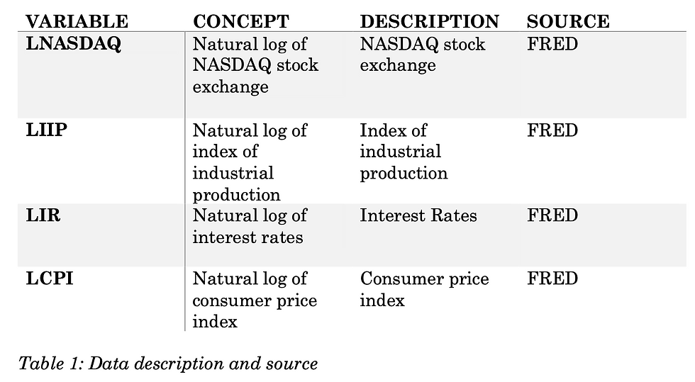
Inflation

Inflation is measured by fluctuations in the US Consumer Price Index (CPI), obtained from the FRED database. High inflation rates can erode the purchasing power and decrease disposable income, therefore reducing consumer spending and a decline in corporate earnings. This, in turn, can decrease investor confidence and potentially cause a decline in stock prices. Moreover, central banks often respond to rising inflation by implementing tighter monetary policies to curb excessive economic growth and mitigate the potential negative effects of inflation, resulting in higher nominal risk-free rates and in turn, higher discount rates. High inflation exerts negative effects on corporate profits, leading to a decrease in dividend payouts. This decline subsequently lowers the expected return on stocks, contributing to a depreciation in their value. Conversely, lower inflation rates translate to more favourable borrowing costs, enhanced corporate performance, increased production and profitability and higher dividend payments by companies. The monthly inflation in this study was computed as the natural logarithm of consumer price index at time t.

Interest rate

This study uses the 10 year Treasury Bill rate as a proxy for interest rates as Treasury bill serves as a benchmark for measuring interest rates and was obtained from the FRED database. Empirical investigations by scholars such as Chen et al. (1986), Abugri (2008), Gan et al. (2006), have provided evidence of the relationship between interest rates and stock returns. Elevated interest rates contribute to increased cost of borrowing for businesses which can in turn reduce investment and expansion endeavours. This can dampen corporate profits, future cash flows and dividend payments, leading to a downward pressure on stock values. Therefore, it is anticipated that interest rates will exhibit a negative relationship with stock market returns.

Index of industrial production

The index of industrial production is used as a proxy for real economic activity. As an indicator of economic activity, industrial production reflects the health and growth of industries within a country. When industrial production rises, if often signifies economic growth, leading to higher corporate profits and increased investor confidence. These combined factors contribute to an increase in stock prices. Conversely, a decline in industrial production can indicate economic contraction, lower profits, and reduced investor optimism, leading to potential decreases in stock values. Therefore, industrial production's impact on stock prices is closely tied to broader economic trends and business performance.

NASDAQ Share Index

The research incorporated the NASDAQ Share Index as a representation of the state of the US Stock Market. The NASDAQ Share Index, functioning as a comprehensive market indicator, evaluates the overall stock market performance. This index is formulated by the NASDAQ Stock Exchange. The calculation of the NASDAQ Share Index involves taking the natural logarithms of the index's values at month t.

3.2 The APT model

The study employs a three-variable APT model to explore the potential correlation between the chosen macroeconomic variables and stock returns. Originating from the work of economist Stephen Ross in 1976, APT emerged as an alternative to the Capital Asset Pricing Model (CAPM). APT is an effective tool for capturing the dynamic relationships among economic factors and stands as a comprehensive framework for asset valuation. The multi-factor nature of the model allows for the analysis of various factors that may influence stock returns, with each factor being assessed by its specific beta coefficient. This approach enables to investigate how inflation, interest rates, and industrial production could contribute to fluctuations in stock returns. The APT model used in this study is expressed as follow:

𝐥𝐧(𝑵𝑨𝑺𝑫𝑨𝑸) = 𝜷𝟎 + 𝜷𝟏 𝐥𝐧(𝑪𝑷𝑰) + 𝜷𝟐 𝐥𝐧(𝑰𝑰𝑷) + 𝜷𝟑 𝐥𝐧(𝑰𝑹) + 𝜺 (3.1)

• ln(NASDAQ) denotes the natural logarithm of the stock market return, serving as the dependent variable.

• ln(CPI) signifies the natural logarithm of inflation rate, serving as one of the independent variables.

• ln(IIP) stands for the natural logarithm of the index of industrial production, serving as another independent variable.

• ln(IR) represents the natural logarithm of the interest rate, serving as an additional independent variable.

• The error term (ε) representing unobserved factors influencing the stock return not captured by the model.

  
  

  3.3 Econometric Methodology:

• 
  

  The econometric methodology employed in this study outlines the approach adopted to achieve the research objective. The study utilises econometrics techniques to unravel the relationship between the macroeconomic variables under investigation. Before selecting the suitable econometric technique for estimation, an initial analysis of the data is conducted. 3.3.1 Stationarity

  
  

  The core premise of time-series regression hinges on the concept of stationarity. In simpler terms, a time series is considered stationary when its statistical attributes, such as mean and variance, remain consistent over time. Moreover, the covariance between two time intervals relies solely on the time gap between them rather than the specific time points involved in the calculation (Gujarati, 2011, pg.216-217).

  Mean constant: E (𝑌 ) = 𝜇 𝑡

  Variance constant: E (𝑌 – 𝜇 )2 = 𝜎2 𝑡

  Covariance:𝛾 =E[(𝑌 −𝜇)(𝑌 -𝜇)] 𝑘 𝑡 𝑡+𝑘

However, true stationarity is rarely encountered in real-world financial time series data due to the presence of trends and fluctuations that vary across different business cycles. Within econometric analysis, stationarity doesn't imply perfect stationarity but rather signifies that the data demonstrates an acceptable level of variation.

The significance of stationarity for this study lies in the fact that most statistical principles do not apply to non-stationary time series, and regression analysis tools typically assume stationarity. Overlooking non-stationarity can lead to misleading outcomes. For instance, two variables displaying coincidental movement over time might yield a high 𝑅2 value upon regression, even if they lack any substantive relationship and are completely unrelated. This phenomenon is known as "spurious regression" (Brooks, 2019, pg. 438).

Another critical concern arises when applying non-stationary data. The outcomes derived from a specific time series cannot be generalised to other time periods. This contrasts with stationary data, where a shock in one period produces diminishing effects in subsequent periods. Non-stationary data, however, assumes that a shock persists indefinitely, impacting future time series similarly. This can disrupt the qualities of the OLS estimator, eroding its BLUE (best, linear, unbiased estimator) attributes, thereby rendering regression analysis results unreliable (Brooks, 2019).

Regressing a non-stationary variable on a deterministic trend does not yield a stationary variable. This arises from the fact that non-stationary data, characterised by trends or patterns that change over time, requires specific treatment to transform it into a stationary form suitable for statistical analysis. When non-stationarity is detected in a data series, it must undergo differencing a certain number of times, denoted as 𝑑, to achieve stationarity. This process involves taking the difference between consecutive observations, which helps remove the underlying trend and make the data more stable and predictable. To illustrate this, consider the following equations which represent two unrelated non- stationary variables:

yt = yt−1 + ut ut~IN (0,1) (3.2)

xt = xt−1 + vt vt~IN (0,1) (3.3)

The regression model is estimated as follows:

yt = β0 + β1xt + εt (3.4)

As the coefficient of determination 𝑅2 approaches zero, the logical inclination might be to accept the null hypothesis 𝐻0: 𝛽 = 0. However, due to non-stationary 1 data, assuming that 𝜀𝑡 is also non-stationary could lead to an incorrect assumption of a correlation between the two time series indicated by the regression model. In reality, the two series could be moving in the same direction for different reasons and rates unrelated to each other (Harris, 1995, pg.16). In essence, for non-stationary series, we cannot determine if correlation implies a causal link between the variables, as we could infer from stationary series. Before attempting to transform non-stationary series into stationary by differencing, it's crucial to identify the distinct models characterising non- stationary data.

Two commonly used non-stationary models are the random walk model with drift (3.5) and the trend-stationary process (3.6), where 𝑢𝑡 represents white noise disturbance for both models.

yt = μ + yt−1 + ut 3.5 yt = α + 𝛽𝑡 + ut (3.6)

Both non-stationary models necessitate distinct treatments to "eliminate" non- stationarity. The process of trend-stationary, or deterministic non-stationarity, requires detrending. This involves regressing equation (3.6) and any subsequent estimation on the residuals, effectively removing the linear trend (Chris Brooks, 2019, pg. 338).

The random walk model with drift, often known as stochastic non-stationarity due to the stochastic trend, achieves stationarity through differencing once. This can be done by letting ∆𝑦𝑡 =𝑦𝑡 −𝑦𝑡−1 and 𝐿𝑦𝑡 =𝑦𝑡−1 so(1−𝐿)𝑦𝑡 =𝑦𝑡 −𝐿𝑦𝑡 =𝑦𝑡 − 𝑦𝑡−1. Taking equation 3.5 and subtracting 𝑦𝑡−1 on both sides, produces the following (Brooks, 2002, pg.371):

𝐲𝐭−𝑦𝑡−1 =μ+𝐮𝐭 (1−L)𝐲𝐭 =μ+𝐮𝐭

∆𝑦𝑡 =μ+𝐮𝐭

For the random walk model with drift, 𝑦𝑡 can be viewed as an explosive process 𝑦𝑡 = 𝜇 + 𝜙𝑦𝑡−1 + 𝑢𝑡, where 𝜙>1.A𝜙>1implies that a shock at time 𝑡 will increasingly affect subsequent periods 𝑡 + 1, 𝑡 + 2, and so on, which is not practically viable for this analysis. Hence, for practicality, 𝜙 = 1 is assumed, aligning with its better fit for financial time series. This is termed the unit root case, where the root of the characteristic equation is unity. Alternatively, 𝜙 < 1 implies a gradual fading of the shock's impact over time—depicting stationarity (Brooks, 2019, pg. 338).

3.3.2 Testing for Stationarity

In the context of this research, evaluating whether the time series data under consideration exhibits stationarity or not necessitates employing a combination of both formal and informal methodologies. One fundamental approach, as elucidated by Gujarati, entails a preliminary graphical analysis where trends and seasonal patterns are visually inspected. However, it's important to note that this technique is considered informal due to its inherent subjectivity and potential ambiguity in decisively determining stationarity based solely on visual assessments. As a preliminary step, this graphical analysis is often undertaken before subjecting the data to more rigorous testing.

Another informal technique commonly employed is the Autocorrelation Function (ACF), commonly referred to as a correlogram, which provides a visual representation of how serial correlation changes across different time intervals. This tool aids in assessing the potential presence of patterns or trends in the data over time.

For a more comprehensive evaluation of stationarity, the research turns to formal unit root tests such as the Dickey-Fuller (DF) and Augmented Dickey- Fuller (ADF) tests. The Dickey-Fuller Test is particularly suitable for simpler AR(1) processes, providing insights into whether a given time series possesses a unit root or not. In contrast, the Augmented Dickey-Fuller Test is more versatile, accommodating more complex data generating processes by integrating a greater number of lagged terms into the analysis (Harris, 1995).

In the present study, the assessment of stationarity for key variables, namely the NASDAQ Share Index, Interest Rates, Inflation Rates, and Index of Industrial Production, will rely on the Augmented Dickey-Fuller Test. This test will enable the research to make informed conclusions about the stationarity properties of these variables, thereby establishing a robust foundation for the subsequent analytical stages of the investigation.

3.3.3 Ordinary Least Square (OLS) Estimation

After ensuring the stationarity of the time series data through the unit root testing, the subsequent phase of the methodology involves the application of the Ordinary Least Square (OLS) estimation. OLS is a widely used method in econometric analysis that aims to estimate the coefficients of a linear relationship between the dependent variable and one or more independent variables. In the context of this research, OLS estimation will be employed to quantify the relationships between the selected macroeconomic variables (Interest Rates, Industrial Production, and Inflation) and the Nasdaq stock index, which serves as a proxy for US stock market returns. By fitting a linear model to the data, OLS estimation allows for the determination of how changes in the independent variables correspond to changes in the dependent variable.

Chapter 4 – Data and Analysis

4.1 Descriptive statistics

Table 2 presents a comprehensive overview of the descriptive characteristics of the analysed macroeconomic variables. Each variable's mean return is depicted, and it's noteworthy that all variables, except for interest rates, exhibit positive mean returns. This exceptional behaviour of interest rates points to a consistent downward trajectory or decline observed across the observation period. The "sum squared deviation" row provides valuable insight into the net change experienced by each variable during the sample period. Particularly, it's evident that interest rates have undergone a substantial decline of around 250% throughout the period under investigation.

Turning to the analysis of skewness, NASDAQ Stock Index's return distribution displays positive skewness, indicating that it possesses a longer right tail, suggestive of occasional extreme positive returns. Conversely, the Consumer Price Index, Index of Industrial Production, and Interest rates manifest negative skewness, implying that their return distributions feature extended left tails. This suggests that these variables have experienced a greater frequency of negative returns than what a normal distribution would anticipate.

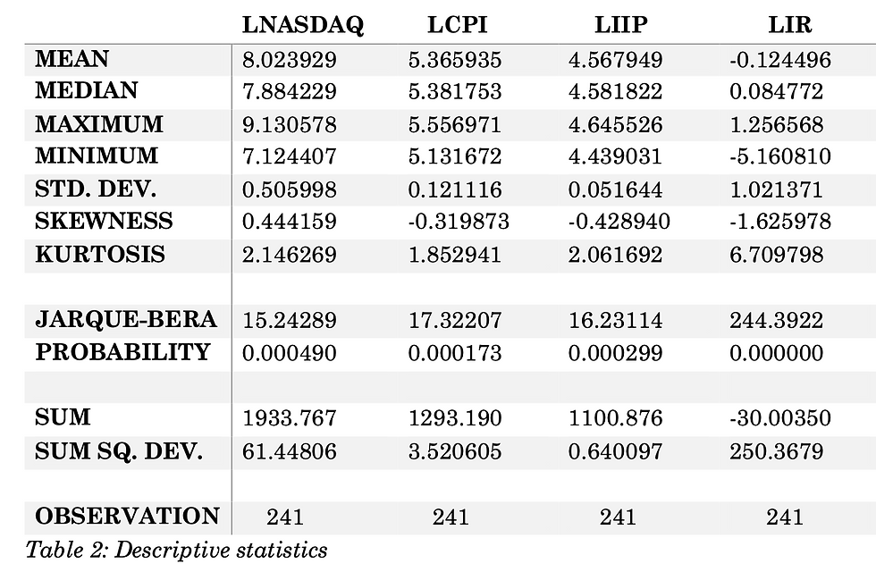
Remarkably, all the variables seem to exhibit a relatively normal distribution, as supported by the p-values derived from the Jarque Bera statistic. This statistic assesses the normality assumption of the variables' distributions. Notably, interest rates exhibit a significantly higher Jarque Bera value compared to the other variables. This divergence could potentially be attributed to a variety of economic and financial factors, encompassing policy decisions, market volatility, and specific market conditions.

4.2 Unit root test results

In order to confirm whether the time series under investigation are stationary, the Augmented Dickey Fuller test is performed on each time series and the results are summarised in table 3. Detailed results for each individual test are available in the Appendix. Consequently, the following hypothesis are evaluated:

𝐻𝑂: 𝛽1 = 0 (𝑡h𝑒 𝑡𝑖𝑚𝑒 𝑠𝑒𝑟𝑖𝑒𝑠 𝑐𝑜𝑛𝑡𝑎𝑖𝑛𝑠 𝑢𝑛𝑖𝑡 𝑟𝑜𝑜𝑡)

𝐻1: 𝛽1 ≠ 0 (𝑡h𝑒 𝑡𝑖𝑚𝑒 𝑠𝑒𝑟𝑖𝑒𝑠 𝑑𝑜𝑒𝑠 𝑛𝑜𝑡 𝑐𝑜𝑛𝑡𝑎𝑖𝑛 𝑢𝑛𝑖𝑡 𝑟𝑜𝑜𝑡)

The ADF test indicates that, with regard to all four series, the null hypothesis 𝐻𝑂: 𝛽1 = 0, suggesting the presence of a unit root, can be rejected. This rejection is supported by the LNASDAQ t-statistic of -11.7210, the LIIP t-statistic of - 4.05870, the LIR t-statistic of -13.4462, and the LCPI t-statistic of -10.5338, all of which exceed their respective critical values (1%, 5%, and 10%) in absolute terms. Consequently, it can be inferred that all four time series exhibit non-stationarity in levels, however, once these series are differenced once, they transition to a state of stationarity.

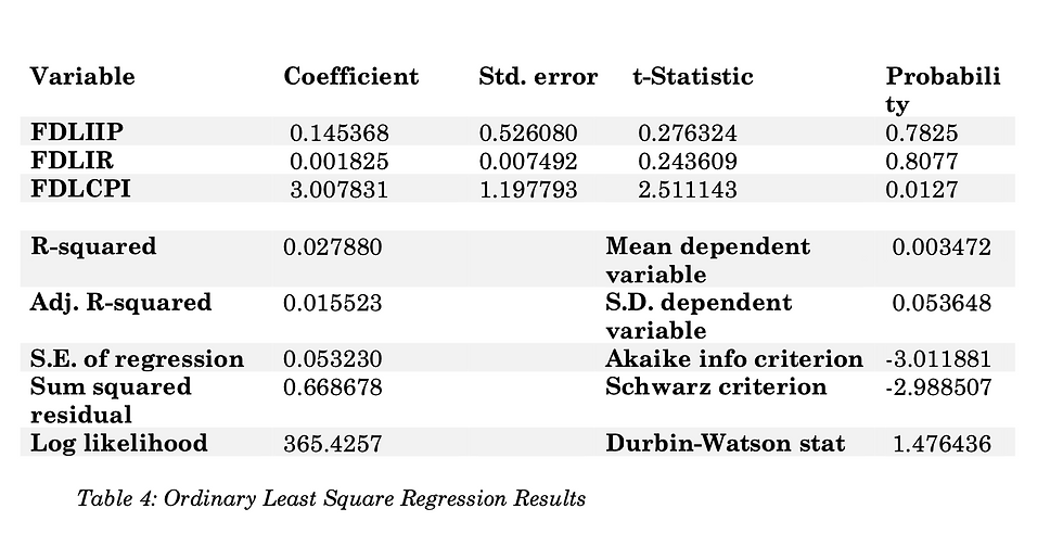
4.3 Ordinary least square regression

The initial outcomes of the regression analysis depicted in Table 4, reveal indications of autocorrelation within the residuals, as implied by the unfavourable Durbin-Watson Statistic score of 1.476436. This value falls short of the desired threshold of 1.5 - 2.0, suggesting the presence of residual autocorrelation. However, after incorporating the autoregressive term, AR (1), into the model the Durbin-Watson Statistic elevates to a satisfactory level of 1.935093, effectively addressing the autocorrelation issue. These changes are highlighted in Table 5 of the analysis.

FDLNASDAQt = β0 + β1t FDLIIPt + β2t FDLIRt + β3t FDLCPIt + AR(1) + εt (4.1)

Where FDLNASDAQt is the first difference of the logarithm of stock market returns; FDLIIPt is the first difference of the logarithm of industrial production; FDLIRt is the first difference of the logarithm of interest rates, FDLCPIt is the first difference of the logarithm of inflation, AR(1) is the incorporated autoregressive term and εt is the error term.

The outcomes of the regression analysis reveal that approximately 7.6% of the fluctuations observed in stock market returns can be accounted for by the three examined macroeconomic variables: inflation, interest rates, and industrial production. This insight is supported by the value of the Adjusted R-squared, which serves as an indicator of how well these variables collectively contribute to explaining the changes in stock market returns.

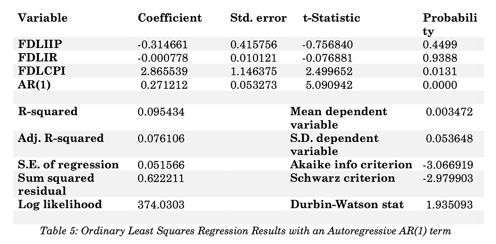
The observed 2.865539 regression coefficient in the analysis indicates a positive relationship between inflation (FDLCPI) and stock market returns (FDLNASDAQ). In simpler terms, this means that when inflation increases, stock market returns tend to increase as well. This positive relationship has been identified by the coefficient, suggesting that for every unit increase in inflation, there is a corresponding increase in stock market returns.

These research findings are in line with prior investigations conducted by Ratanapakorn and Sharma (2007), Pal and Mittal (2011), and Bordo et al.(2008). These studies also found evidence of a positive connection between inflation and stock market returns. This consistency across multiple studies suggests that the relationship between inflation and stock market performance is not an isolated occurrence but rather a recurrent pattern observed in various economic contexts. The positive relationship between inflation and stock market returns might be explained by several factors. One common interpretation is that moderate inflation can reflect a growing economy, potentially leading to higher corporate earnings and increased consumer spending, which in turn can positively influence stock prices. The results from this empirical investigation indicate an interesting trade-off that investors consider between the risks associated with holding stocks and the potential returns they can achieve. This relationship has implications for risk management. Investors often seek investments that can provide adequate returns to compensate for the risks they undertake. In this context, when inflation rises, the value of money decreases over time, and investors aim to ensure that their investments can counteract this effect. Therefore, they might require higher returns from stocks to account for the eroding impact of inflation on their purchasing power. Furthermore, the study's outcomes also highlight a noteworthy aspect related to using stocks as a hedge against inflation. A hedge is an investment that can offset the impact of adverse price movements in another investment. In this case, if stocks were an effective hedge against inflation, their returns would be expected to rise when inflation increases. However, the positive regression coefficient suggests that US stocks might not serve this purpose effectively, as the positive relationship between CPI and stock returns implies that higher inflation rates demand even higher expected returns from stocks. This finding underscores that while stocks can be an investment option, they might not work as an efficient hedge against the negative effects of inflation in this particular context.

The obtained regression coefficient of -0.314661 signifies a weak negative relationship between industrial production (FDLIIP) and stock prices (FDLNASDAQ). In simpler terms, this indicates that when industrial production increases, there's a tendency for stock prices to decrease, though this relationship is not particularly strong. A value closer to zero implies that changes in industrial production have only a minor influence on stock prices in the opposite direction.

These results might appear counterintuitive, as conventional economic theory would often suggest that a thriving industrial sector should lead to increased economic activity and potentially higher corporate profits, which could be associated with higher stock prices. However, the observed weak negative relationship challenges this expectation.

Interestingly, the outcomes of this research contrast with the findings of previous studies. For instance, Gan et al. (2006) reported a positive relationship between GDP (economic activity) and stock prices. This suggests that, according to their analysis, a growing economy was associated with higher stock prices. On the other hand, Abbas et al. (2015) discovered a weak negative relationship between GDP and stock returns, which aligns with the findings of this research. The differing results across studies can be attributed to various factors, including variations in data periods, sample sizes, and methodologies employed. Additionally, the impact of industrial production on stock prices can be influenced by intricate dynamics within the economy, including investor sentiment, market conditions, and the specific sectors that make up the industrial production index.

The outcomes of the regression analysis revealed a relationship that is both statistically insignificant and negative between interest rates and stock market returns, as indicated by the coefficient of -0.000778. This implies that the observed change in interest rates is not associated with a substantial or meaningful change in stock market returns.

This finding aligns with the research of Onasanya and Ayoola (2012), who also discovered a similar negative and insignificant connection between interest rates and stock market returns. Their study, like the present research, concluded that changes in interest rates did not significantly impact changes in stock market returns.

However, there are contrasting viewpoints from studies conducted by Pal and Mittal (2011) as well as Ratanapakorn and Sharma (2007) who reported a positive relationship between stock prices and interest rates, suggesting that when interest rates increase, stock prices also tend to rise. This discrepancy highlights the complexity of the relationship between interest rates and stock market returns, which can be influenced by a multitude of factors and economic conditions. Moreover, these findings can alert investors that changes in interest rates might not have a substantial influence on stock market returns. While interest rates are often considered a key factor in investment decisions, this research suggests that other variables might play a more dominant role in influencing stock market performance. Investors may need to consider a broader set of factors when making investment choices and not rely solely on interest rate movements as a predictor of stock market returns.

Chapter 5 – Conclusions and Recommendations

This paper investigates the effects of macroeconomic variables on the stock market returns in the US. It estimates a multivariate APT model with the dependent variable being NASDAQ share index. In this study, a macroeconomic factor model is employed to test the effects of macroeconomic factors on asset pricing for the period of January 2000 to January 2020. The macroeconomic variables under investigation in this research are inflation, industrial production and interest rates. An OLS regression methodology was employed to establish the relationships between the stock market returns and the macroeconomic variables. In the regression model, the macroeconomic variables were used as independent variables whereas stock market returns were used as dependent variables. Based on the analysis conducted in this study, several significant insights emerge that hold implications for investors and policymakers alike. Firstly, the findings from this empirical analysis reveal a positive relationship between inflation (CPI) and stock market returns which means that as inflation rises, so do stock market returns. This observation points to a compelling dynamic that investors weigh when making decisions – a balancing act between the inherent risks linked to holding stocks and the potential rewards they can attain. In simpler terms, when inflation goes up, the general cost of goods and services tends to rise over time. To safeguard the value of their investments against this decline in purchasing power, investors seek assets that can generate returns surpassing the rate of inflation. Secondly, the weak negative relationship identified between industrial production (IIP) and stock prices (NASDAQ) signifies that, though counterintuitive, when industrial production increases, there's a tendency for stock prices to decrease. While this relationship might seem contrary to conventional economic theory, it highlights the intricate dynamics at play. Investors should approach this relationship with a more nuanced perspective, recognising that the connection between industrial production and stock prices is influenced by various factors, including investor sentiment, market conditions, and the specific sectors that constitute industrial production. Thirdly, the insignificant and negative relationship found between interest rates and stock market returns indicates that changes in interest rates might not have a meaningful impact on stock market performance. This conclusion is consistent with the research of Onasanya and Ayoola (2012), revealing that shifts in interest rates do not significantly affect stock market returns. This insight can guide investors by suggesting that other variables might have a more substantial influence on stock market performance, encouraging them to consider a more comprehensive set of factors when making investment decisions. Policymakers can also take note that changes in interest rates might not always have a significant ripple effect on stock market returns, encouraging a broader consideration of economic strategies.

While this study examines three significant macroeconomic variables, it's essential to recognise that the selected variables represent only a small portion of the potential factors at play. The inclusion of additional relevant macroeconomic indicators holds the potential to yield a more extensive comprehension of the relationship between economic dynamics and stock market returns, thus opening up avenues for future research endeavours.

To enhance the robustness and accuracy of assessing the influence of macroeconomic variables on stock market returns, upcoming research might consider adopting advanced methodologies such as vector error correction and cointegration analysis. These techniques provide distinct advantages by offering insights into both short-term and long-term estimations, enabling a deeper understanding of the intricate connections between macroeconomic forces and stock market performance. The implementation of such advanced methodologies can pave the way for future investigations in this domain. Bibliography

1. Abbas,S.,Tahir,S.H.andRaza,S.,2015.Impactofmacroeconomic variables on stock returns: Evidence from KSE-100 Index of Pakistan. Research Journal of Economic and Business Studies, 3(7), pp.70-77.

2. Abdullah,D.A.andHayworth,S.C.,1983.MacroeconometricsofStock Price Fluctuations. Journal of Business Economics, 32(1), pp.49-63.

3. Abugri,B.A.,2008.EmpiricalRelationshipbetweenMacroeconomic Volatility and Stock Returns: Evidence from Latin American markets. International Review of Financial Analysis, 17, pp.396-410.

4. Aljandali,A.andTatahi,M.,2018.Economicandfinancialmodellingwith eviews. A Guide for Students and Professionals. Switzerland: Springer International Publishing.

5. Anokye,M.A.andTweneboah,G.,2008.MacroeconomicFactorsandStock Market Movement: Evidence from Ghana. Munich Personal RePEc Archives, p. 11256.

6. Bordo,M.D.,Dueker,M.J.andWheelock,D.C.,2008.Inflation,Monetary Policy and Stock Market Conditions: Quontitative Evidence from a Hybrid Latent-Variable VAR. Federal Reserve Bank of St. Louis Working Paper Series.

7. Brooks,C.,2002.IntroductoryEconometricsforFinance.Cambridge University Press. 1st Edition.

8. Brooks,C.,2019.Introductoryeconometricsforfinance.4thed. Cambridge: Cambridge University Press.

9. Bulmash,S.B.andTrivoli,G.W.,1991.Time-laggedInteractionsbetween Stock Prices and Selected Economic Variables. Journal of Portfolio Management, 17(4), pp.61-67.

10. Cecchetti, S.G., 2008. Crisis and responses: the Federal Reserve and the financial crisis of 2007-2008 (No. w14134). National Bureau of Economic Research.

11. Chen, N.F., Roll, R. and Ross, A.S., 1986. Economic Forces and the Stock Market. Journal of Business, 383-403.

12. French, K.R., Schwert, G.W. and Stambaugh, R.F., 1987. Expected Stock Returns and Variance. Journal of Financial Economics, 19, pp.3-29.

13. Gan, C., Lee, M., Yong, H. and Zhang, J., 2006. Macroeconomic Variables and Stock Market Interactions: New Zealand Evidence. Investment Management and Financial Innovations, 3(4), pp.89-101.

14. Gujarati, D., 2011. Econometrics by example. 1st ed. London: Macmillan Education Palgrave.

15. Gupta, R. and Reid, M., 2013. Macroeconomic surprises and stock returns in South Africa. Studies in Economics and Finance, 30(3), pp.266-282.

16. Harris, R., 1995. Using cointegration analysis in econometric modelling. Hemel Hempstead, England: Harvester Wheatsheaf, Prentice Hall.

17. Jecheche, P., 2006. An Empirical Investigation of Arbitrage Pricing Theory: Case of Zimbabwe. Research in Business and Economic Journal.

18. Kraay, A. and Ventura, J., 2007. The dot-com bubble, the Bush deficits, and the US current account. In G7 Current Account Imbalances: Sustainability and Adjustment (pp. 461-462). University of Chicago Press.

19. Lintner, J., 1965. The valuation of assets and the selection of risky investments in stock portfolios and capital budgets. Review of Economics and Statistics, 47, pp.13-37.

20. Onasanya, O.K. and Ayoola, F.J., 2012. Does macroeconomic variables have effect on stock market movement in Nigeria. Journal of Economics and Sustainable Development, 3(10), pp.192-202.

21. Ouma, W.N. and Muriu, P., 2014. The impact of macroeconomic variables on stock market returns in Kenya. International Journal of Business and Commerce, 3(11), pp.1-31.

22. Pal, K. and Mittal, R., 2011. Impact of Macroeconomic Indicators on Indian Capital Markets. Journal of Risk Finance, 12(2), pp.84-97.

23. Premawardhana, V., 1997. The relationship between stock returns and interest rates in Sri Lanka.

24. Ratanapakorn, O. and Sharma, S.C., 2007. Dynamic analysis between the US stock returns and the macroeconomic variables. Applied Financial Economics, 17(5), pp.369-377.

25. Ross, S.A., 1976. The Arbitrage Theory of Capital Asset Pricing. Journal of Economic Theory, 341-360.

26. Rjoub, H., Türsoy, T. and Günsel, N., 2009. The effects of macroeconomic factors on stock returns: Istanbul Stock Market. Studies in Economics and Finance, 26(1), pp.36-45.

27. Malpezzi, S., 2017. Residential real estate in the US financial crisis, the Great Recession, and their aftermath. Jing Ji Lun Wen Cong Kan, 45(1), pp.5-56.

28. Maysami, R.C., Howe, L.C. and Hamzah, M.A., 2004. Relationship Between Macroeconomic Variables and Stock Market Indices: Cointegration Evidence from Stock Exchange of Singapore's All-S Indices. Journal of Pengurusan, 24, pp.47-77.

29. Menike, L.M.C.S., 2006. The effect of macroeconomic variables on stock prices in emerging Sri Lankan stock market.

30. Mossin, J., 1966. Equilibrium in a capital asset market. Econometrica: Journal of the Econometric Society, pp.768-783.

31. Naik, P.K., 2013. Does Stock Market Respond to Economic Fundamentals? Time Series Analysis from Indian Data. Journal of Applied Economic and Business Research, 3(1), pp.34-50.

32. Sharpe, W.F., 1964. Capital asset prices: A theory of market equilibrium under conditions of risk. Journal of Finance, 19, pp.425-442.

33. Smart, S.B., Gitman, L.J. and Joehnk, M.D., 2017. Fundamentals of Investing (Vol. 13). Malaysia: PEARSON.